Swapping pgvector for turbopuffer made our whole database faster and cheaper

Learn how our shared pgvector table made our smallest customers the slowest, why an HNSW index made it worse, and how moving to turbopuffer made our whole database faster and cheaper.

Like many other AI products, Modem uses embeddings. When new customer messages come in, we want to know whether any customers have said something similar before, in any channel and in any wording. Embeddings are part of how we answer that.

When we started off, we wanted to manage as few moving pieces as possible. So those embeddings lived in Postgres with the pgvector extension. And for a long time it was fine.

Then our searches started getting slow in a way that made no sense. Some of our smallest customers waited up to ten seconds for results while our biggest customers (with the most data to scan) got answers immediately. And the whole time our database compute costs soared.

In this post, I'll explain what was slowing us down, why the standard fix didn't work for a product like ours, and how we eventually capitulated and switched to turbopuffer, which cut our p90 search time by 76% and took most of the load off our database.

Why we started on Postgres

Modem reads the places your team and users talk (support tickets, issue trackers, call transcripts, Slack) and groups what it finds into topics. Every time it pulls a new customer concern out of a conversation, it asks the database: has any customer said something like this recently?

To answer that, we use embeddings. An embedding is a long list of numbers, called a vector, that a model produces from a piece of input text. Strings that mean similar things get vectors that point in similar directions.

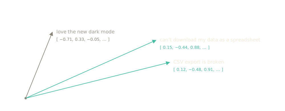
When we started out, we had very little data, and didn't bother indexing our embeddings. So to do this query, Postgres looked at the customer's recent rows and compared every one of them against the new embedding.

This brute force approach worked for much longer than it should have. Our database provider, Neon, had generously gifted us free compute credits, which let us overprovision instead of optimize, so we did. And because these vector searches ran in a number of background jobs as part of data ingest, the slow queries were mostly imperceptible to users.

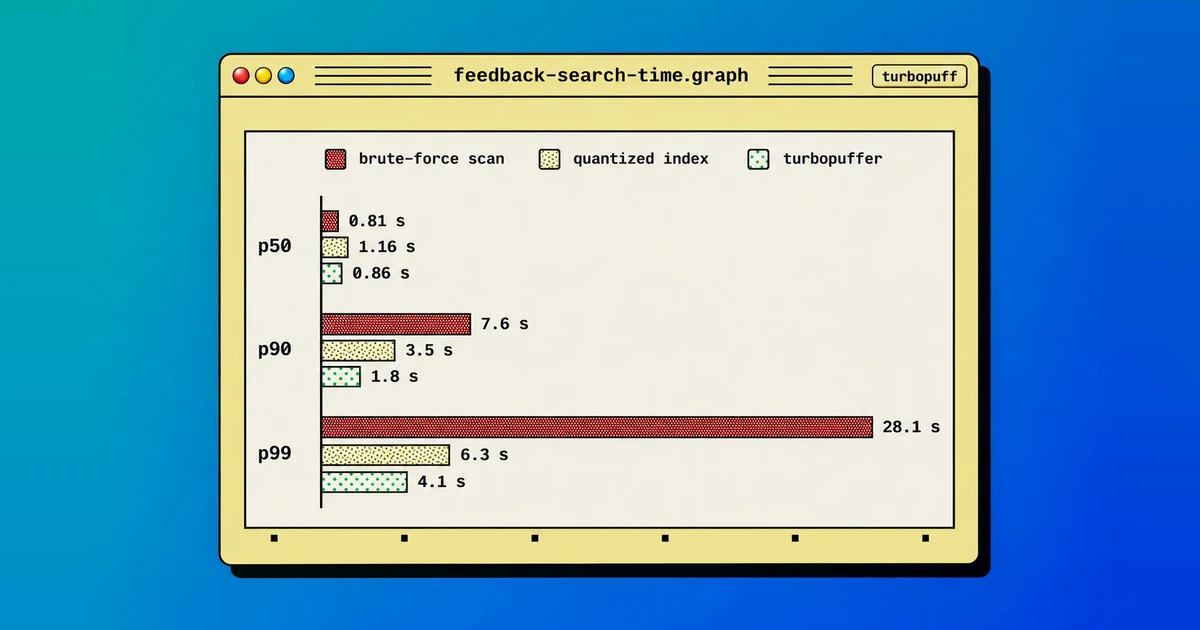
But as we added more customers and ingested more data, the number of embeddings began growing rapidly. By August 2026, the median search took about 0.8 seconds and the slowest 1% took as long as 28 seconds. Our Neon compute kept scaling to keep pace, and a surprising amount of that was this one query. Eventually our free credits ended, the database bill came due, and we quickly realized what kind of problem we were sitting on.

The standard fix for a slow query in a database is adding an index. But during testing, not only did this index not improve performance, it made it materially worse.

How HNSW indexes work

The standard vector index in pgvector is HNSW, which stands for Hierarchical Navigable Small World. It's supported by many vector databases, and it's how vector search gets fast.

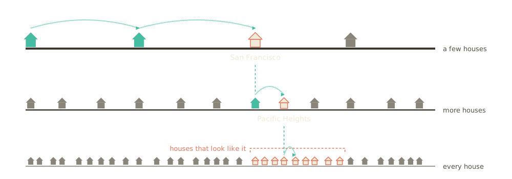
Instead of comparing your query against every row, HNSW builds a graph where each vector links to its nearest neighbors, stacked in layers from sparse to complete. A search starts at the top, hops toward whatever is closest, drops a layer, and repeats. You look at a few hundred rows instead of the whole table, and the answer is approximate but usually very good.

Let me give you an example. Imagine you're given a picture of a house, and asked to find a set of houses that look like it. You'd start with a handful of houses spread across the world and go to the one that looks most like your picture.

Say that first hit is a house in San Francisco. Then you'd look at more houses around San Francisco, closer together, and move to the one that looks most like it, which might put you in a neighborhood like Pacific Heights. Finally you'd walk the streets there until you're surrounded by houses that look like your picture. That's roughly how HNSW finds similar vectors.

Surprise: HNSW can make performance worse

If HNSW can answer your query on its own, it's great. But our query had two extra filters:

• the organization_id the data belongs to
• a time range (for recency)

Normally, Postgres combines indexes for you. You have one index for organization_id, one for timestamp, and the planner pulls the matching rows from each, keeps the rows that belong to both, and moves on. This all just happens and you don't have to think about it.

SELECT ... FROM semantic_groups
WHERE organization_id = $org_id        -- Organization filter
  AND timestamp > now() - $time_window -- Time range
ORDER BY embedding <=> $candidate
LIMIT $count;

But HNSW doesn't work that way. A regular index answers "which rows match?" HNSW answers "which rows are closest?" And "closest" applies to everything in the vector space, ignoring any other filters. Put another way, Postgres walks the graph across the whole table first and applies your regular column filters afterwards.

On a multi-tenant table shared by lots of customers, that's a disaster. The vector query returns a fixed number of candidate matches from the entire table, then the organization_id and time filters throw out everything that doesn't belong to the target org or time range. Often this means candidate results that start out promising are reduced to an empty set.

Back to the house search example. Say you still want to find houses that look like the input image, but you have a new condition: you only want to consider houses for sale. You do the same search as before: San Francisco, Pacific Heights, a street full of houses that look like your picture. Only then do you check for signs. None of those houses are for sale, so you come back with nothing, even though a few houses down the street were.

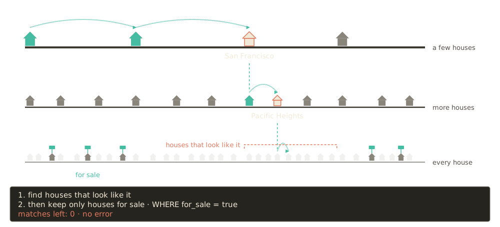
This is a known issue with pgvector. So much so it has a setting, hnsw.iterative_scan, that keeps widening the walk until enough rows survive the filter.

We tested it against the brute-force scan on a few thousand real production searches.

• Customers with fewer than 500 groups got 89× slower at the median, 9.1 seconds versus 103 ms.
• About 7% of results changed, including dozens of matches a person had previously confirmed were related.
• The worst search took 178 seconds.
• The indexes nearly doubled the table's storage.

The smaller the customer, the more of the graph the walk has to wade through to find its rows. And because we're a self-serve product with a free tier, most of our customers are small.

So we took the index back out and went back to the brute-force scan. That still left the original question. Why was it so slow in the first place?

Why our smallest customers were the slowest

As we kept digging, we made a strange discovery.

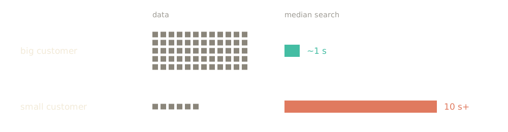
A big customer sending us feedback all day had a median retrieval time of ~1s. A much smaller customer that sent us data periodically had a median above 10s. This felt backwards because in database land, it's more typical to see slower queries associated with large accounts (with more data to scan).

So what was going on?

The busy customer and the quiet customer were running the exact same query. The difference was where their data happened to be when the query ran.

Postgres keeps recently used data in memory, and every customer shares that memory. Our embeddings were big enough that only a small slice of them fit in memory at once. The busy customer searched often enough to keep its rows in memory. The quiet customer came back to find its rows pushed out by everyone else, so every search went to disk.

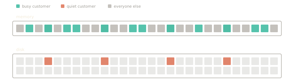
The scan itself was fine. It always gave the right answer. The trouble was that every row was expensive to read, and most of them now came from disk.

One last try: shrinking the vectors to fit in memory

By now we doubted pgvector would keep up with Modem's growth. We just wanted to buy ourselves time before we'd need to swap infrastructure.

If HNSW wasn't going to work, and the issue was that our embeddings were too big to stay in memory, could we create an alternative index, using much smaller quantized embeddings?

The thesis was that a sufficiently small vector index could remain entirely in memory, with nothing on disk. So we went as small as you could possibly go: binary quantization.

pgvector has a function for this, binary_quantize(), that shrinks an embedding by keeping only whether each of its 1,536 numbers is positive or negative. This is represented using a single bit, 1 or 0.

embedding  [ 0.021, -0.013,  0.008, -0.044,  0.017,  0.030, -0.002, ... ] // N = 1,536
quantized  [     1,      0,      1,      0,      1,      1,      0, ... ] // N = 1,536

That reduces 3 KB into 192 bytes, and comparing two of them is a fast bit count instead of 1,536 multiplications. This obviously loses a lot of precision. But, because the embeddings take up so much less space, and comparisons are so fast, you can overfetch and compare a much larger set of candidates.

Back to the house example one last time. It's like flipping quickly through a stack of tiny, blurry photos of every house, choosing a bunch that roughly look right, then driving up to see if those matches are actually a fit.

We kept these quantized embeddings in their own small table, and it fit in memory with room to spare. And because this is just a regular Postgres table, we could index columns like organization_id and timestamp so the query planner makes an efficient query the way you'd expect.

So every search looked like this:

1. Compare against every one of the customer's recent quantized embeddings and keep the closest N candidates, where N is roughly 50x the actual target you want to finish with.
2. Run our original exact query on the full precision embeddings, but only for that shortlist.

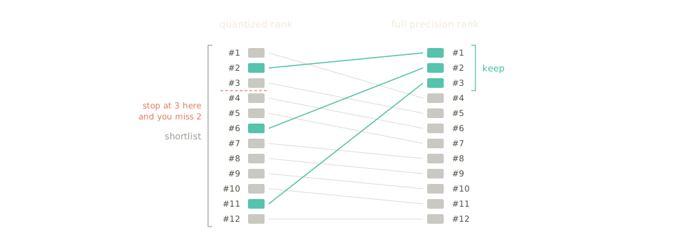
It worked. A replay harness ran thousands of real production searches both ways, and the quantized index returned the same results as the brute-force scan. It also cut the tail. Over a week of production traffic, p90 dropped from 7.6 s to 3.5 s and p99 from 28.1 s to 6.3 s. The median went the other way, from 0.81 s to 1.16 s, but the slow searches were the ones causing trouble.

This was a real win. Searches got faster and the results didn’t change. But the full halfvec embeddings were still in Postgres, and even with the shortlist, each search had to read a lot of them. Keeping those reads fast meant keeping them in memory, so we were still paying for far more database than the rest of the app needed. In other words, the query got faster but our Neon bill didn’t get smaller.

Moving to turbopuffer

That's when we stopped trying to make pgvector happen.

It was time to do what - in our hearts - we knew had to be done all along: switch to a dedicated vector database solution. We went with turbopuffer.

turbopuffer is a proprietary search database created in 2023 by two former Shopify engineers, offered as a paid SaaS service. It does vector and full-text search, and keeps everything on object storage like S3, with memory and SSD caches in front for the data being searched right now. That makes it cheap to keep a lot of vectors around and fast to search the ones you're using.

turbopuffer fixes both halves of our problem. It handles the filters where they belong, inside the search and not after it. And it keeps the embeddings out of Postgres, in a system built around the idea that most vectors are cold most of the time.

Each customer gets its own namespace, so their vectors live in their own index. So right off the jump we are only looking at the customer's search space. And this has the added benefit of providing better data isolation between accounts.

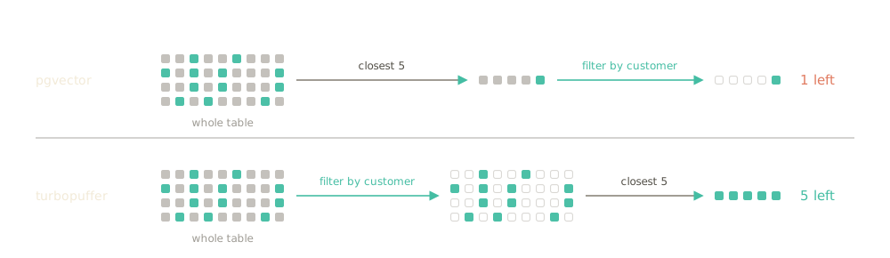
We store a timestamp on every vector, so turbopuffer only searches the ones inside the time window. pgvector's HNSW index can't do that. It finds the nearest rows first and checks their dates afterwards, and an iterative scan keeps looking until enough of them pass. Our quantized table got the dates right, but it had to compare against every row in the window to do it.

Rolling it out

The switch itself was small, because of the month we'd spent on the quantized index. Our search already ran in two steps: build a shortlist, then rank it exactly. And we had the replay harness to tell us whether a shortlist was any good. All we changed was where the shortlist came from.

We wrote every vector to both systems and ran every customer in shadow mode. Postgres still answered for real, and turbopuffer ran the same search alongside it so we could compare every result. 88% came back identical. Another 11% had small differences, like two nearly equal matches coming back in a different order.

The last 1% came mostly from customers with one huge topic. Hundreds of messages about the same thing would fill a search and crowd everything else out. Asking turbopuffer for one result per topic fixed it, and what was left (0.43%) were ties between equally good matches.

The results

Once we were confident, we switched everyone over. Here's the search time for each new piece of feedback under all three approaches, each measured over about a week of production traffic.

The median barely moved, because most searches were never the problem. The tail is where it changed. Against the brute-force scan, p90 fell 76% and p99 fell 85%: the slowest 10% of searches got about four times faster, and the slowest 1% almost seven times faster.

A note on these numbers. They're the full round trip as our pipeline sees it, network included, not the time the database spends on the query. And some of our searches ask turbopuffer for exact results, which means comparing against every one of the customer's recent rows, so those take longer the more that customer has. For a background job we'd rather be right than fast.

Here's the week of the switch, hour by hour.

Note that at this point, Postgres was slower than when we initially introduced our quantized index. The table had grown, and we'd added a second search for a new feature, one that still ran as a brute-force scan and competed for the same memory. This illustrates why we needed a better long term solution; writing a hack fix around one query pattern didn't account for new queries we'd introduce along the way.

What it did for Postgres

Postgres got its memory back. Over the first 24 hours, CPU on our production database dropped 62%, cache misses dropped 82%, and slow queries on the table dropped 95%. Everything else in Postgres got faster too, because this expensive vector query stopped occupying all of the memory. We were able to downsize our Neon DB instance and reduce our database bill.

Even though we were also now paying for turbopuffer, switching to this dual system dropped our entire storage bill - serving all Modem data, not just embeddings - by roughly 10%.

What we'd do differently

None of this was the plan. We started out wanting one database and ended up with two.

We'd still start on Postgres. One database is less to run, and brute force over a small table is fine for longer than you'd think. But looking back, three things would have gotten us here sooner:

Check who is slow, not just how slow. Our median looked fine. It was only when we split search time by customer that we saw the small, quiet ones waiting ten times longer. If your slowest searches belong to your smallest customers, look at memory before you look at the query.

Test an index against real searches before you trust it. HNSW with a filter can return different results, or fewer, and nothing errors. We only caught it because we ran it against real production searches and compared the answers. Build a harness for that first. Ours outlived every approach in this post.

Count what the vectors cost the rest of your database. The quantized index made our searches fast enough. What it couldn't do was stop the embeddings from crowding everything else out of memory, and we were paying for that overprovisioning the database.

What fixed it was moving the embeddings somewhere they don't compete with the rest of our data for memory.

One more database turned out to be simpler than one more filter.